New York City
Airbnb pricing analysis
and prediction
This project examines the extensive dataset of New York City Airbnb listings. Exploratory data analysis is conducted to identify patterns and trends in host demographics, property availability, and key metrics. Additionally, prediction algorithms are utilized to estimate rental prices based on factors such as location, property type, and amenities. The objective is to offer valuable insights for hosts, guests, and stakeholders in the tourism industry, aiding in pricing strategies and investment decisions within the dynamic NYC Airbnb market.

Context
Airbnb has transformed the hospitality landscape, offering travelers unique accommodations and experiences while empowering hosts to monetize their spaces. Analyzing Airbnb data provides valuable insights into market dynamics and informs decision-making for hosts, guests, and stakeholders. This project focuses on exploring the NYC Airbnb market and predicting rental prices to guide pricing strategies and investment decisions.
Content of the dataset
The dataset, sourced from Inside Airbnb, contains comprehensive information on NYC Airbnb listings. It includes details on host demographics, property characteristics, geographical availability, and rental metrics. Each feature provides valuable insights into the NYC Airbnb landscape, facilitating exploratory analysis and predictive modeling.
Acknowledgements
The dataset can be accessed on the Inside Airbnb website. Users can navigate the website to locate the NYC dataset and download it for analysis. The used dataset was a modified version of the original dataset mentioned provided by the company Indicium. Prior to analysis, data preprocessing and cleaning are recommended to ensure the dataset is ready for exploratory analysis and predictive modeling.
Used technologies
In the analysis and prediction of trends within the NYC Airbnb listings dataset, Jupyter notebooks and essential Python libraries such as pandas, matplotlib, seaborn, wordcloud, and scikit-learn were employed.
Exploratory data analysis (EDA)
Understanding the dataset
To carry out the exploratory data analysis, data from the dataset provided was investigated. The file has 48.894 rows and 16 columns. Each column is described below.
- id - Acts as a unique key for each ad in the application data
- name - Represents the name of the ad
- host_id - Represents the id of the user who hosted the ad
- host_name - Contains the name of the user who hosted the ad
- neighborhood_group - Contains the name of the neighborhood where the ad is located
- neighborhood - Contains the name of the area where the ad is located
- latitude - Contains the latitude of the location
- longitude - Contains the longitude of the location
- room_type - Contains the type of room for each ad
- price - Contains the price per night in dollars listed by the host
- minimum_nights - Contains the minimum number of nights the user must book
- number_of_reviews - Contains the number of comments given to each listing
- last_review - Contains the date of the last revision given to the listing
- reviews_by_month - Contains the number of reviews provided per month
- calculated_host_listings_count - Contains the number of listings per host
- availability_365 - Contains the number of days the ad is available for booking
It was then possible to check which variables are categorical and which are quantitative, as shown in the table below.
| Categorical variables | Quantitative variables |
|---|---|
| id | latitude |
| name | longitude |
| host_id | price |
| host_name | minimum_nights |
| neighborhood_group | number_reviews |
| neighborhood | reviews_by_month |
| room_type | calculated_host_listings_count |
| availability_365 | |
| last_review |
Next, information related to the dataset was analyzed in order to understand its format and the quality of the data. The characteristics analyzed were the number of unique entries in each column, the number of zero values in each column and the number of duplicate rows. All these factors appeared to be normal, so there was no need to perform data cleaning at this point.
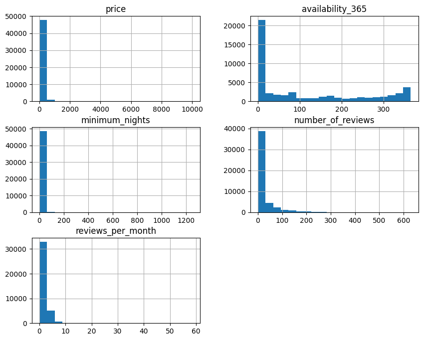
The distribution of the numerical variables was observed to get more information about the data. Table 2 was generated containing statistical data for each column.
| price | availability_365 | minimum_nights | number_of_reviews | reviews_by_month | |
|---|---|---|---|---|---|
| total | 48,894 | 48,894 | 48,894 | 48,894 | 38,842 |
| average | 152.72 | 112.78 | 7.03 | 23.27 | 1.37 |
| std | 240.15 | 131.62 | 20.51 | 44.55 | 1.68 |
| min | 0 | 0 | 1 | 0 | 0.01 |
| 25% | 69 | 0 | 1 | 1 | 0.19 |
| 50% | 106 | 45 | 3 | 5 | 0.72 |
| 75% | 175 | 227 | 5 | 24 | 2.02 |
| max | 10,000 | 365 | 1.250 | 629 | 58.5 |
As you can see, the price and minimum_nights columns stand out. The price column has an average of 152.7, but a maximum value of 10,000. It also has values equal to zero. With regard to the minimum_nights column, its average is 7.03, but its maximum value is 1250. This leads us to conclude that there are outliers that should be dealt with when cleaning the data.
To visualize the distribution of the data, histogram-type graphs were plotted, showing once again that the price and minimum_nights columns are poorly distributed. The histograms are shown in Figure 1 below. The other columns appear to be correct according to interpretation.
Identifying outliers and data cleaning
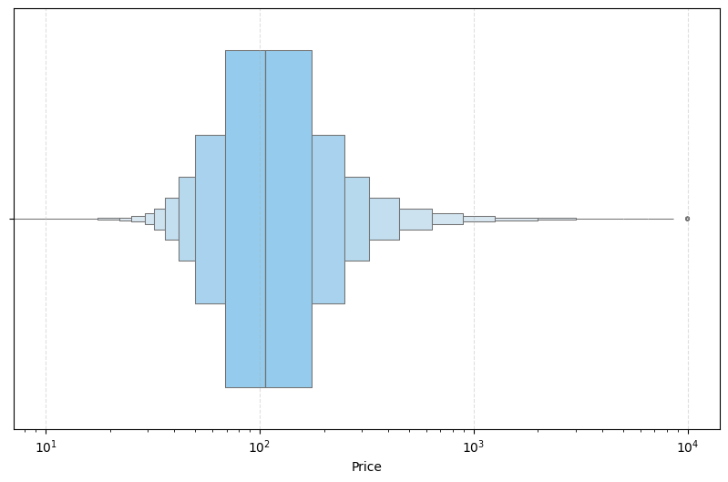
To identify the outliers in the price and minimum_nights variables, boxenplot graphs were used, which are similar to boxplots, but because they have more quantiles, it is possible to better analyze the distributions in the tail, where the outliers are present. Firstly, the graph was plotted for price, where it was identified that from US$600 onwards, the values did not contribute and could distort the analysis. They represent only 1.59% of all listings, and the values where the price is zero only 0.02%. You can also see that more than 50% of the values are in the range of US$70 and US$110. A logarithmic scale was used on the x-axis to make the visualization clearer. The boxenplot for price is shown in Figure 2.
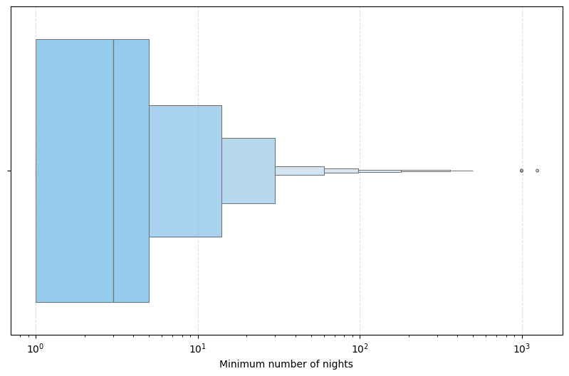
The second box plot was the minimum number of nights, shown in Figure 3. It shows that 50% of the values are between 0 and 4 nights, and the values above 30 nights, which represent only 1.53% of the total listings, can influence the quality of the analysis.
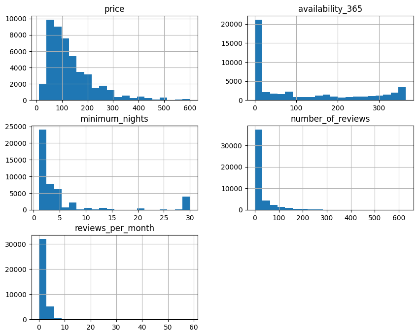
Once the outliers had been identified, the data was cleaned, generating a new table containing listings for prices other than zero and less than US$600, as well as minimum nights of less than 30 days. To check that the data cleaning was effective, new histograms were plotted for the variables in question, as shown in Figure 4. As you can see, the price and minimum nights distributions are much clearer.
Room type analysis
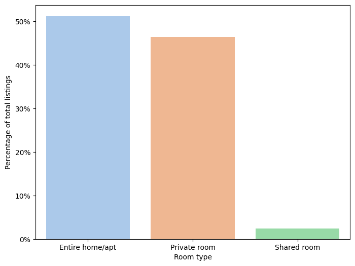
Once the data has been cleaned, data analysis can begin. The first attribute to be analyzed is room type. In Figure 5, which shows the percentage of listings for each type of room, you can see that the Entire home/apt category is the one with the most listings, accounting for over 50% of them. This is followed by the Private room category, with approximately 48%, and finally the Shared room category, with approximately 2%.
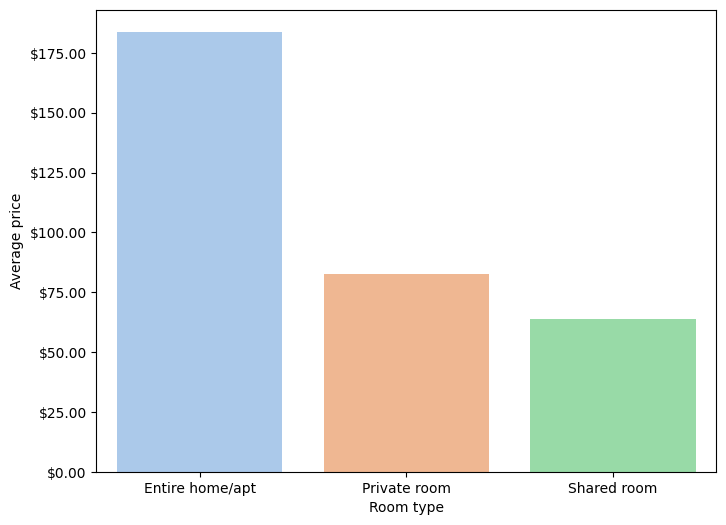
The next graph in Figure 6 shows the average price of each type of room. The highest average price is in the Entire home/apt category, with an average value of approximately US$185, followed by the Private room with an approximate value of US$80 and finally the Shared room with an approximate value of US$65. With this, we can see that there is a big difference between the value of an entire apartment/home and the other two categories.
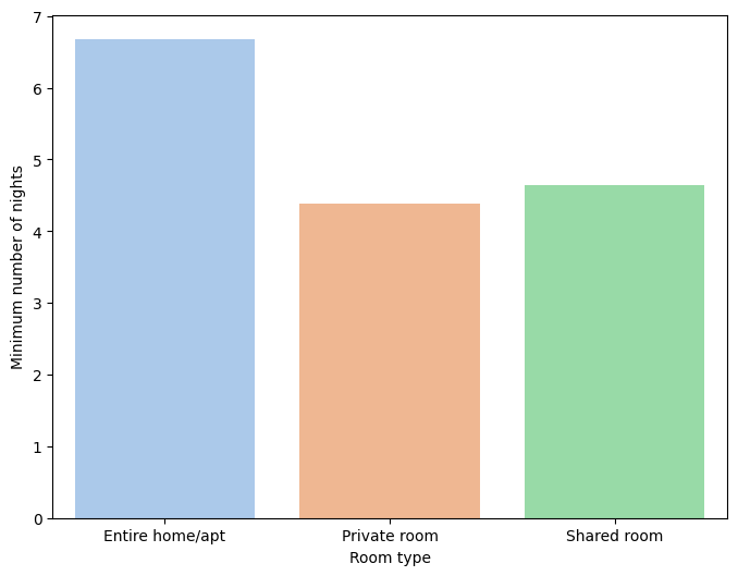
The following graph, shown in Figure 7, shows the average number of minimum nights for each type of room. The type of room that has the highest average is Entire home/apt, with almost 7 nights, followed by Shared room, with approximately 4.7 nights, and finally Private room, with an approximate average of 4.5 nights.
Neighborhood analysis
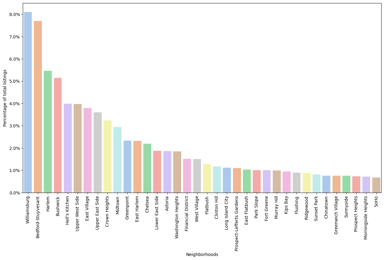
The next attribute to be analyzed was neighborhoods, where there are a total of 221 possible options. Because of the large number of neighborhoods, it was decided to use only the neighborhoods that represent 80% of the listings, i.e. 36 neighborhoods. Figure 8 shows the percentage of listings per neighborhood. It shows that the three neighborhoods with the highest number of listings are Williamsburg, Bedford-Stuyvesant and Harlem, accounting for approximately 21% of all listings.
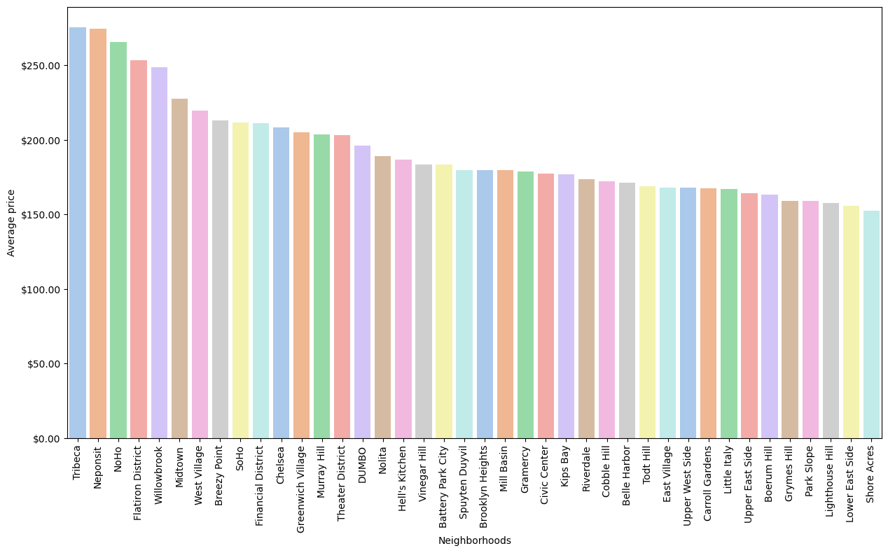
The average price of each neighborhood was also analyzed for the 36 selected neighborhoods, as shown in Figure 9. It can be seen that the Tribeca, Neponsit and NoHo neighborhoods have the highest average values, reaching over US$250.
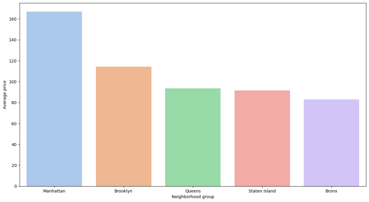
The neighborhood groups were also analyzed to identify the average price in each neighborhood group. In Figure 10, you can see that Manhattan has the highest average price of over US$160, almost double that of the Bronx. The neighborhoods that follow and their respective approximate values are Brooklyn at US$110, Queens at US$95, Staten Island at US$90 and finally the Bronx at US$80.
Correlation between variables
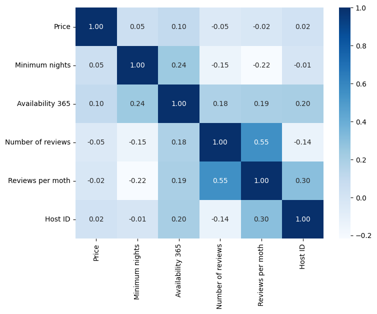
To identify the relationship between certain variables, the correlation index was used. Correlations were calculated for the following variables: price, minimum_nights, availability_365, number_of_reviews, reviews_per_month, host_id. A heat map containing the correlation values between the variables was then plotted, as shown in Figure 11. It can be seen that they all have a low correlation with each other. The only variables that have a significant level are the number_of_reviews and reviews_per_month, which makes sense since one depends on the other. You can also see that the correlation between price and the other variables is very low, showing that they don't interfere in setting the price.
Spatial analysis
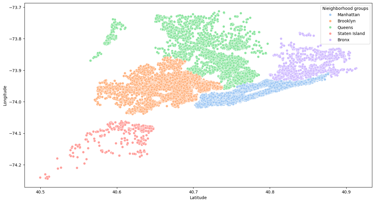
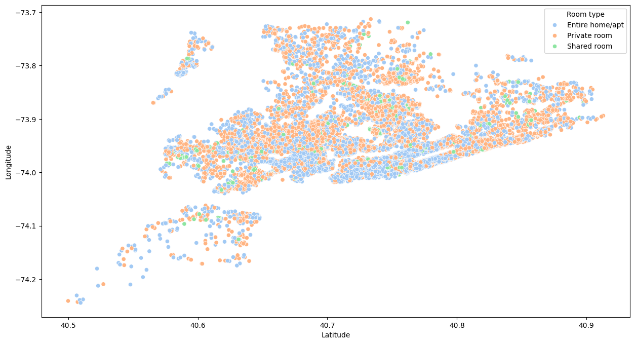
The next analysis was of the spatial distribution of ads by type of room and by neighborhood group. Figure 12 shows the distribution of neighborhoods according to latitude and longitude, where you can see that the fewest ads are in the Bronx and Staten Island, and the most ads are in the other three boroughs.
In Figure 13, you can see that there are a large number of private room and apartment/house ads scattered around the city. It also shows that there are few shared room listings in the dataset.
Listings names analysis
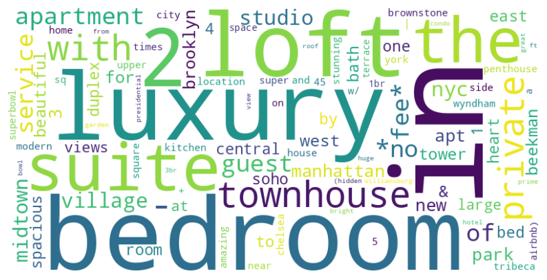
Finally, the last analysis was of the ad names. As these are texts without defined formatting, the best way to identify patterns is to use word clouds. This tool creates graphic representations based on words and their frequency of occurrence in a text. The larger the word in the image, the more often it appears in the text. With this tool, it is possible to identify the words that appear most often in ads. The analysis was carried out for high-value ads, over US$600, and the word cloud in Figure 14 was generated. As you can see, some words do not represent patterns for higher-value ads, since they are common words in real estate ads. Some words stand out when it comes to identifying high-priced ads, such as: luxury, large, spacious, penthouse. These words are relevant and are common in higher-value ads.
Price prediction
Price forecasting can be seen as a regression problem, since the aim is to estimate a numerical value rather than a category. Therefore, two regression algorithms were chosen: multiple linear regression and random forests.
The two models were based on three categorical variables (neighborhood, neighborhood_group and room_type) and one quantitative variable (price). These were chosen because, as shown in the exploratory data analysis, they have a direct effect on the price of advertised properties. In order to use the categorical variables in the models to be built, it was necessary to create dummy variables.
The performance measures chosen were root mean square error (RMSE) and the coefficient of determination of the test and training datasets (R2). The RMSE was chosen because it provides an estimate of how well the model is able to predict the value in question, and is used to assess accuracy. The coefficient of determination was chosen because it determines the proportion of the variance in the dependent variable that can be explained by the dependent variable, i.e. how well the data fits the regression model.
Multiple linear regression
For the linear regression, the data was separated into test and training, with proportions of 20% and 80% respectively, assigning the categorical variables to x and the price to y. With this, the model was trained and had a score of 0.43 when applied to the test dataset.
To assess the model's performance, the measures mentioned above were calculated. The mean square error was 68.16. The R2 coefficient for testing and training was 0.43 and 0.41 respectively.
Random forests
For the random forests, the data was also separated into test and training, with proportions of 20% and 80% respectively, assigning the categorical variables to x and the price to y. With this, the model was trained and had a score of 0.42 when applied to the test dataset.
To assess the model's performance, the measures mentioned above were calculated. The mean square error was 68.46. The R2 coefficient for testing and training was 0.42 and 0.41 respectively.
Choosing the best model
Based on the results, you can choose the model that best matches the data. As you can see, the mean square error values and the R2 coefficients are similar for the two models, which shows that they are equivalent in this type of classification.
The model can also be chosen according to its characteristics. The advantages of using linear regression are better interpretability and computational efficiency, making it suitable for smaller and less complex data sets. The disadvantages are its possible rigid assumptions and sensitivity to outliers, limiting its applicability. The advantages of the random forest algorithm are its high precision and robustness against outliers, dealing well with non-linear and complex relationships in the data. Its disadvantages are that it is less interpretable and may require adjustment of hyperparameters. Thus, for the case of this dataset, both models are effective.
Predicting a value
To make the price suggestion, the values were predicted using the models created. The information to be included in the forecast is shown in the code snippet below.
										{'id': 2595,

										'name': 'Skylit Midtown Castle',

										'host_id': 2845,

										'host_name': 'Jennifer',

										'neighborhood_group': 'Manhattan',

										'borough': 'Midtown',

										'latitude': 40.75362,

										'longitude': -73.98377,

										'room_type':

										'Entire home/apt',

										'price': 225,

										'minimum_nights': 1,

										'number_of_reviews': 45,

										'last_review': '2019-05-21',

										'reviews_by_mes': 0.38,

										'calculated_host_listings_count': 2,

										'availability_365': 355}
The variables used were neighborhood, neighborhood group and room type. Applying these values to the algorithms resulted in the prices US$252.94 and US$222.76 for the multiple linear regression and random forest models respectively. As you can see, the value that comes closest to the real value is that of the random forest algorithm.